- Innovations
- Articles on application of PCI
- New Trading Horizons
Pair Trading with Inverse Spread: 3 Steps
Those who already faced the Trend Following concept know that effective strategies of following the trend suggest dynamic stop loss level movement without profit limitation. The position is kept until the trend is changed and the order is done. With a proper choice of the market entry point the trader switches a position into the breakeven mode and thus relieves the psychological pressure. With this approach, a profit limitation is deliberately not applicable, allowing holding the position for a long time. This approach is also useful as it minimizes the commission fee calculated on the intraday basis that the trader pays to the broker. The Trend-Following strategy uses the market momentum and allows taking profit in the long-term and large-scale trends.
The natural obstacles to this strategy are the long term low volatility in the selected time frame (sideways movement), as well as systematic sudden market changes. We would like to show you a method of pair trading with inverse spread by the example of Personal Composite Instruments - PCI that allows finding new areas of sustainable trend occurrence and hedging systematic risks at the same time.
Step1. Fundamental hypothesis
Pair trading involves using two competitors belonging to one market segment. The opposition of their values allows minimizing systematic, i.e. market risks. In the table below, we have some examples of correlated pairs listed: COFFEE/COCOA, F/GM, FCATTLE/SOYB, Google/Apple, NATGAS/BRENT. Trading each of these pairs within the NetTradeX trading platform is carried out formally as a cross currency pair trading, for example EUR/CHF. Nevertheless, using correlated pairs allows reducing the risks associated with food market, car market, or high-tech commodity market. Ideally, when both of assets have the same sensitivity to the market, the spread pair is neutral and depends only on the comparative asset performance.
For example, let us assume that the demand for high-tech products had fallen significantly due to the global economy recession. If we had an open long position on Google, this would fatally lead to a negative transaction balance. If the GOOG/AAPL volume was bought, then both assets would decrease in value, but at the same time, their cross-rate may grow. This can happen in case of higher stability of the Google Company against systemic risks than its competitor’s.
| Base instrument | Quoted instrument | Market segment |
| Coffee/COFFEE | Cocoa/COCOA | Food |
| Ford Motor/F | General Motors/GM | Automotive industry |
| Beef/FCATTLE | Soybean/SOYB | Food |
| Apple | Hi-Tech | |
| Natural gas /NATGAS | Oil/BRENT | Natural resources |
Table 1. Examples of correlated pairs
Here we assume that the assets have a normal relation, i.e. the growth of the base and the quoted assets are positively correlated. Indeed, if the growth in the food market is observed for a long time, this will fatally lead to the higher prices of coffee and cocoa. At the same time, we do not take the competition into account. The influence of systemic factors is noticeable on monthly longer term scales. We would like to consider the principles of high-frequency trading: W1, D1 or less.
For this purpose, we consider the anomalous relation of competing assets. All the instruments indicated in the table can belong to this group. We are looking for a simple interpretation of the fundamental situation where the competition would have a sharp effect.
Example 1:
Using soybeans as a meat substitute, ceteris paribus can create a unique situation where the demand for these two products is replaceable. In case of constant supply, it can lead to inverse relation between the #C-FCATTLE beef futures price change and the #C-SOYB soybean futures. As the supply is inertia and reacts slowly to the food fashion relatively to the demand (production capacity, staff, etc.), it can be assumed that such a situation arises regularly. So, our hypothesis is: in case of stable market supply and substitution demand, rise in soybean futures prices provokes the decrease of the frozen beef futures in value and vice versa. Which way to turn, it depends on consumer income (soy is a cheaper substitute), healthy diet fashion, vegetarian fashion, feeding costs, etc.
The mechanism of all other fundamental factors is not important for trading, as we can consider only comparison factors. Using the method of pair trading with inverse spreads allows significantly simplifying the fundamental analysis (!).
Example 2:
Consideration of the mixed spread of competing assets such as shares of Coca-Cola #S-KO and futures for frozen concentrated orange juice #C-ORANGE is also interesting. It is worth to note that in volume terms natural orange juice is on average 1.5-2 times more expensive at the moment than carbonated beverages produced by the Coca-Cola Company. It is no surprise that the orange juice concentrate consumption decreased by 14.7% in the crisis beginning and in the period of 2007-2012. And this happened when the Coca-Cola Company revenues started growing faster than they did before the crisis, reaching a 50% growth within 2007-2012. If we compare the growth of the #S-KO price and orange concentrate futures, we will see the situation is sharper. So the #S-KO stocks raised by 46% vs. 2.6% for #C-ORANGE.
The demand substitution effect is most clearly manifested in the healthy lifestyle macro trend strengthening. The opposite situation is possible when the fast food demand grows, for example, during systemic economic crisis. One of these tendencies may lead to inverse relation increase for the #S-KO and #C-ORANGE.
Step 2. Statistical hypothesis testing: asset movement correlation
After figuring the main hypothesis out, we try to find the optimum market situation where the position on the pair instrument could be opened. Our task is to determine the period where the inverse relation between the dynamics of competing assets is expressed in the sharpest way. The pair correlation coefficient can be used as the simplest indicator.
The r correlation shows the linear dependence degree of the analyzed assets. The r coefficient is located in the range [-1,1], or from -100% to 100%, in terms of percentage points. When the values are close to 100% the dependence of the price change for the assets can be approximately described by the following equation:
ΔA 2 = ΔA 1 * k (1)
Here we have ΔA 1 as the absolute price change of the Asset 1 and ΔA 2 as the absolute price change of the asset 2. In this case, the k coefficient is a positive constant: k > 0.
For negative values of the k < 0 key correlation the base asset price growth leads to the quoted asset price fall and vice versa. Thus, if the rcoefficient is close to -100%, the price changes are expressed by the same equation, but k < 0. This is the case that is the most interesting for spread trading competing assets. At the same time, a small deviation of the spread pair prices leads to the further movement in this direction - the synthetic instrument has a predisposition to the trend - this effect will be explained below.
To find the inverse spread we use the indicator of the (r) correlation coefficient attached to the main chart of the instrument in the MetaTrader 4 platform. For example, if we have the #S-KO/#C-ORANGE cross pair considered, then, we open the The Coca-Cola Company daily price chart in the upper window. Then we set the Ind_Correlation.mq4 indicator in the window below. We specify the first asset in the parameters regardless the order, then the second asset and the time period we calculate the correlation coefficient for – i.e. the number of bars required for statistical analysis. The statistical volume is primarily determined by the investment horizon and corresponding parameter of other indicators.
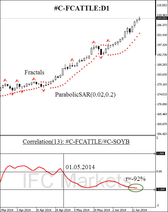
In the FCATTLE/SOYB (frozen beef /soy) cross pair example considered below (frozen beef / soy), we use the 13-days period. Since May 2014, the indicator signal dropped below the critical level of 0% to -92% in early June. We will consider the asset pair having a correlation coefficient less than 0% as an inverse spread. The presented chart confirms the inverse relation of assets on the 13-day horizon and it allows counting on the intensive trend movement.
Here we consider the price change of the cross pair composed as the ratio of the # S-KO base asset price and the corresponding price of the # C-ORANGE quoted asset, providing that both assets have a correlation coefficient close to 100% (eg, below 90% ):
In case of the base asset price increase within the analyzed period, and the quoted asset price fall according to (1), the inverse spread absolute price change is expressed by the equation (3):

Figure1. The correlation between the movement of futures prices for frozen beef and soybeans
The numerator corresponds to the relative change in prices of the quoted asset ΔA1. Thus, the price volatility of the pair instrument is higher than the corresponding relative volatility of the quoted asset α time:
The closer the correlation coefficient to the - 100% limit value, the higher the pair instrument volatility vs. the quoted instrument volatility is. The α - effect is what allows using the trend-following strategy more effectively and quitting the sideways corridor as quickly as possible.
But what does make the trend movement sustainable after the corridor is left? Let us assume that the correlation of ΔA2 and ΔA1 is close to -100%, while the quoted asset price leaned down for fundamental reasons: ΔA2< 0. This will fatally lead to the rise in prices of the base asset A1 and the α coefficient respectively. A small deviation of one of the assets leads to a nonlinear volatility increase and the trend beginning. In this situation, the trend following strategy becomes effective.
Step 3. Pair instruments technical analysis and a position opening
In the Figure 1, we can see that crossing the critical level of 0% correlation was recorded in May 1st, 2014. Before May 14th, the coefficient has been falling down to the historic low at 92%, which fatally led to the pair instrument volatility increase on the ratio (3) basis. The volatility increase led to refreshment of highs/lows and opening new positions to start following the trend.
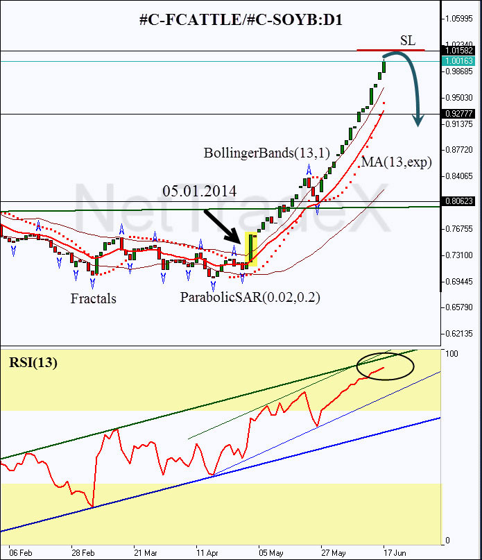
The figure 2 shows the #С-FCATTLE/#C-SOYB daily chart, built within the NetTradeX trading platform. Here we used the PCI technology of Portfolio Quoting Method technology. Composing the instrument took 10 minutes, and 7 mouse clicks. You can find more detailed instructions of composing the PCI instrument here.

Figure2. The FCATTLE/SOYB synthetic instrument chart: D1
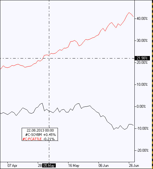
Please note that the Bill Williams fractal, defining the key resistance, was broken through on May 5th (!). This means that the reverse spread growth is determined by substitution in the demand fundamental mechanism that has inertial characteristics. The percentage price change in the # C-FCATTLE and #C-SOYB chart confirms it. In the figure3, we see that the main PCI price growth driver is frozen beef. However, the pair instrument growth rate gets accelerated unlike the #С-FCATTLE elemental instrument. This is due to the alpha - effect influence, discussed above, as the correlation coefficient is close to 100%. A long position could be opened after crossing the resistance and zero correlation levels. Thus, the correlation indicator is used as an additional oscillator or filter, so to speak.
The further trend following occurs by the means of moving the stop loss level in the trend movement direction. We can choose a new Bill Williams bullish fractal, or move the stop loss following the ParabolicSAR indicator. Once the price crosses the stop loss level, the position is closed. A similar situation occurs in case of opening a short position on the PCI.
We also use the Ind Correlation oscillator for closing a position forcedly. Once the indicator value returns to the upper semi plane of positive values, we quit the market. This strategy is necessary for several reasons. Firstly, only negative values make the instrument work more effective than any of the elementary instruments included in the spread. Secondly, only negative correlation values make hedge of systematic risks effective.

Figure 3. The FCATTLE/SOYB synthetic instrument chart.
Indeed, let us assume that the commodity futures market experiences system changes occurred (the humanitarian crisis, recession of the world economy, etc.), which leads to a sudden drop in demand for grains and meat. In this case, each of the traded instruments is determined by the change of the market index :
ΔA1=ΔM0 * β1ΔA2=ΔM0 * β2 (5)
Each of the β1 and β2 proportionality coefficients is a positive number.
The relation between the absolute yields is expressed by the equation (6):
This situation is obviously impossible for retroactive pair assets defined by the ratios (1-3). In this regard, using the reverse spread correlation analysis allows effectively hedging the systemic risks and preventing dangerous situations on the market.
Previous articles
- The Exchange Rate and the Creation of New Financial Instruments on its Base
- Profiting in bear and bull oil markets
- Currency indices: unveiling central banks’ secrets
- Portfolio Trading Method – Expanding the Range of Trading Instruments
- Portfolio Quoting Method – New Ways for Analysis of Financial Markets
- Portfolio Quoting Method - New Trading Strategies
